I try to answer the following questions: could AI could a double in output in 10 years? Then I ask if this holds for 10X and 100X.

I’m just trying to ask what’s feasible, given arbitrarily strong growth in AI capabilties.

It requires breaking it down in a series of subquestions.

First we have to define output growth, when there’s asymmetric growth in different goods. We will say there’s growth of 2X if people are . we define growth in “output” not by average by a factor Y not that average is as good as increasing today’s consumption by a factor of Y. Avg household expenditure is $80K, so 10X growth means we live in a world which is as good as increasing your expenditure to $800K in today’s world.

Q1: Could productivity grow by 2X? Yes.
Q2: Could welfare grow by 2X? Yes.
Q3: Could demand limit output growth? Unlikely.
Q3: Could frontier productivity grow by 2X in a decade? Yes.
Q4: Could average productivity grow by 2X in a decade? Yes.

Could AI double productivity?

Concretely: could productivity, averaged across sectors, grow by 10X?

Historical productivity growth has been enormous in some sectors:

lighting: 500,000X labor efficiency (Nordhaus)
agriculture: 400X labor efficiency
compute: >1000000X cost efficiency (Moore’s law)
LLMs: >700X cost efficiency (NanoGPT)

In each of these cases it seems reasonable to expect more orders of magnitude of efficiency growth available.

AI can increase labor efficiency in two ways: (1) discover new techniques that are more efficient; (2) use the same techniques but replace labor, e.g. drive our cars, harvest our wheat, fill out our spreadsheets and reply to our emails.

Worth noting that the sectoral impact of AI seems different from prior technologies. Clasically productivity growth has been highest in agriculture and manufacturing; but AI seems more likely to have the biggest effect on services, specifically cognitive services: clerical, legal, administrative, medical, teaching (at least in the short run).

Could AI double output?

What does it mean to say that welfare (or output) has increased by 10X, if the composition changes?

If we have 10X increase in welfare or output (using them interchangeably) this means everyone lives as well as they would if they increased expenditure by 10X. Average US consumption is around $80K/year, so we’re asking if AI could make people feel as if they’re living at $800K today.

This would fail if productivity growth was concentrated in sectors with strong diminishing returns. E.g. suppose productivity in manufactured goods went to the moon, such that the average person coulc now afford manufactured goods that would cost $800K in the old prices. This doesn’t give you a standard of living worth $800K if there are sufficient diminishing returns to manufactures.

This point is sometimes called “Baumol effects” or “weak links” or “bottlenecks.”

A reason for optimism is that we have historical precedents for 10X output growth despite productivity gains being concentrated. Our standard metrics of real GDP say that we have grown 10X over the past 120 years (at 2% growth).

(Note: a naive calculation could say that LLMs have already increased output by 2X for some people. E.g. I’m consuming services that would’ve cost me more than $100,000 without AI: getting expert medical advice, writing large programming projects, etc.)

Equivalent variation / compensating variation

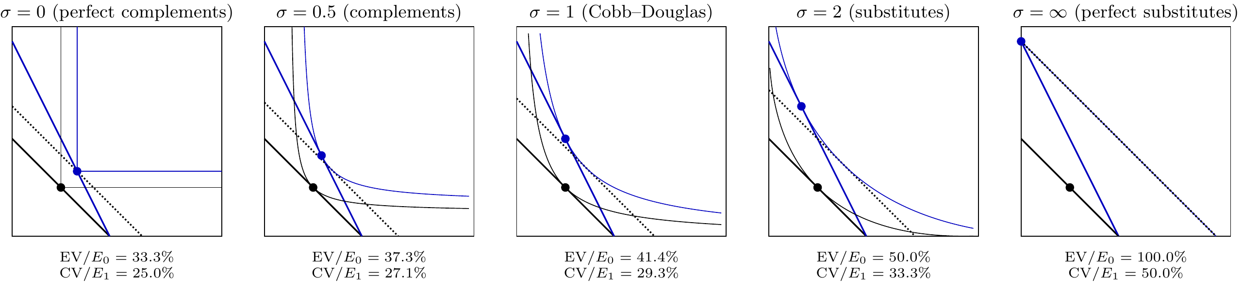
Suppose there are two goods, equal expenditure on each, and the price of good $y$ halves. We can illustrate what happens with different elasticities of substitution. If we observe the quantities and prices, and assume CES, then we can infer the income-equivalent growth (Equivalent Variation, EV).

The same AI price reduction with five elasticities of substitution. Black denotes the pre-AI frontier and indifference curve; blue denotes the post-AI frontier and optimum. The dotted line is the old-price budget shifted outward until it reaches the post-AI utility level.

With perfect complements, both goods rise together. With Cobb–Douglas preferences, expenditure shares remain equal, so $x$ is unchanged and $y$ doubles. With substitutes, the household shifts expenditure strongly toward the now-cheaper $y$, and consumption of $x$ falls. With perfect substitutes, the post-AI household buys only $y$; at the old equal prices every bundle on the initial budget was optimal, and the figure selects the equal-expenditure bundle $(1,1)$.

Equivalent variation values the utility gain at pre-AI prices, while compensating variation values it at post-AI prices:

\[ \frac{\mathrm{EV}}{E_0} =\frac{e(p_0,u_1)-e(p_0,u_0)}{e(p_0,u_0)} =\frac{u_1}{u_0}-1, \qquad \frac{\mathrm{CV}}{E_1} =\frac{e(p_1,u_1)-e(p_1,u_0)}{e(p_1,u_1)} =1-\frac{u_0}{u_1}. \]

Might demand limit AI output?

Is there a sense in which productivity growth could fail to turn into output or welfare growth due to demand?

One sense is that the point above: concentrated productivity growth and diminishing returns.

However there’s also another sense.

Could frontier productivity grow by 10X in a decade? YES.

: - For the task-automation channel, this is just a question of capabilities: if we have AI that can replace people at the computer & operating machinery then we immediately have huge jumps in labor productivity.

- We have historical precedents for 3X output growth over a decade in East Asian countries. However Alwyn Young has argued that this wasn't due to productivity growth, but rather reallocation of labor from low-productivity agriculture to high-productivity manufacturing.

Q: Could we have 10X average productivity growth in a decade? YES.

In what senses ccould demand limit output growth?
What’s the standard rough decomposition of historical output growth into productivity and sectoral change?
Does the answer to these questions change meaningfully if we reduce everything to labor productivity, vs introducing capital and automation?

notes

dogmas of growth economics.

Aggregate productivity has grown ~2%/year over 200 years (50X/year).
Growth has been unbalanced: agriculture > manufacturing > services; labor and expenditure shares shifted towards the lower-growth sectors. (has been disputed how to reconcile structural change with flat aggregate growth).
Aggregate productivity growth is a weighted average of sectoral growth rates.

Growth in output/capita: 2% over 200 years (50X increase)

Growth in productivity:

4% in goods
1% in services

Structural change puzzle.

There’s a classic puzzle in growth theory, how to reconcile (1) big shift from goods to services; (2) roughly constant aggregate growth (Kaldor facts).

Some explanations: (1) substitution (Baumol; Ngai-Pissarides); (2) income effects (Kongsamut-Rebelo-Xie, Boppart); (3) combination (Comin, Lashkari and Mestieri).

Review: Herrendorf et al. (2013) Growth and Structural Change

Productivity growth.

Labor productivity in agriculture up 200X.

	share 1800	share 2000	Δ share	Δ productivity	Δ output
agriculture	75%	2%	1/40	400	10
manufacturing	5%	10%	2	100	200
services	20%	90%	5	10	50

Bread and circuses model.

Empirical income and price elasticities

The closest empirical objects to the parameters in the diagrams are sectoral expenditure elasticities

\[ \eta_i=\frac{\partial\log(p_i c_i)}{\partial\log E} \]

and the elasticity of substitution $\sigma$. In the CES papers, $\sigma$ is a common Hicksian/Morishima elasticity between sectors, not a separate Marshallian own-price elasticity for agriculture, manufacturing, and services. ``Estimated’’ below means directly fitted to data; several foundational papers instead choose or calibrate $\sigma$.

Study and sample	$\sigma$	$\eta_a$	$\eta_m$	$\eta_s$	Interpretation notes
@kongsamutRebeloXie2001beyond	$1$	—	$1$	—	Assumed Cobb–Douglas/Stone–Geary preferences; $\eta_a<1$ and $\eta_s>1$, with both varying by expenditure.
@ngai2007structural	$0.30$ ($0.10$)	$1$	$1$	$1$	Homothetic CES. The first value is the baseline calibration; the parenthetical value is the lower-elasticity sensitivity case.
@acemogluGuerrieri2008capital	$0.76$	—	—	—	Estimated for two value-added sectors grouped by capital intensity, not agriculture/manufacturing/services; two-SE interval $[0.73,0.79]$. Both grouped sectors have expenditure elasticity $1$.
@bueraKaboski2009traditional	$0.50$	—	—	—	Three-sector U.S. calibration. Generalized Stone–Geary expenditure elasticities vary with expenditure.
@duarteRestuccia2010role	$0.40$	—	—	—	Calibrated manufacturing–services elasticity ($\rho=-1.5$). Agriculture is a necessity and services a luxury, with elasticities varying by expenditure.
@herrendorfRogersonValentinyi2013perspectives (final expenditure)	$0.85$	—	—	—	Estimated Stone–Geary specification. Agriculture is a necessity and services a luxury; elasticities vary with expenditure.
@herrendorfRogersonValentinyi2013perspectives (consumption value added)	$0.002$	—	—	—	Estimated and approximately Leontief; elasticities vary with expenditure.
@boppart2014structural	$0.50$	—	$0.70$–$0.80$	$1.12$	Two-sector goods/services model; $\eta_g$ is shown in the $\eta_m$ column. $\sigma$ is its asymptotic value; the service estimate is for 2009.
@cominLashkariMestieri2021structuralchange (U.S. CEX households)	$0.26$	$0.37$	$0.83$	$1.20$	Direct estimates for the average household; SE of $\sigma$ is $0.04$.
@cominLashkariMestieri2021structuralchange (39-country panel)	$0.57$	$0.56$	$1.03$	$1.14$	Direct estimates for the average country-year.

The strongest directly comparable evidence is therefore Comin, Lashkari, and Mestieri’s: $\eta_a<\eta_m<\eta_s$ and $\sigma<1$ in both micro and macro data. The wider literature also usually uses or estimates $\sigma<1$, but values are not directly comparable when papers use value-added sectors, two-sector aggregates, homothetic preferences, or calibration rather than demand estimation.