
There are a lot of cute thought experiments where the apparent value of something depends on what it’s compared to:
- A \$5 discount off a \$20 radio feels more valuable than a \$5 discount off a \$500 bed.
- The difference between a 1% chance and a 2% chance seems more important than between a 51% chance and a 52% chance (likewise with 1 and 2 days vs 51 and 52 days).
- Paying \$10 for a liter of ice cream seems more attractive if you see that the price of half-liter is \$8
- (I list some more examples at the bottom).
Many people have felt that there’s a common principle at work, in particular: that the sensitivity to an attribute (price, probability, square feet) depends on the set of quantities that you’re considering. But different people have proposed different principles:
- Range: sensitivity is decreasing in the range of values observed, i.e. you’re less sensitive as the difference between the maximum and minimum increases: Volkmann (1951), Mellers & Cooke (1994), Bushong Schwarzstein & Rabin (2016).
- Negative Range: sensitivity is increasing in the range of values observed, the exact opposite of the above: Koszegi & Szeidl (2003).
- Proportional Range: sensitivity is increasing in the proportional range of values (the range divided by the average): Bordalo Gennaioli & Shleifer (2013).
- Frequency: sensitivity at any point is increasing in the density of values in that neighborhood: Parducci (1965), Stewart Chater & Brown (2010).
- Magnitude: sensitivity is decreasing in the magnitude of the values (e.g. the average): my own paper: Cunningham (2015).
- There are lots of other variants, most notably ones with a reference point, e.g. Loss Aversion says you’re more sensitive below a reference point, and Diminishing Sensitivity says you’re more sensitive in the neighborhood of a reference point (both are in Tversky & Kahneman 1991)..
All of these models can be thought about as indifference curves that change slope as you change the elements in the choice set, e.g. below adding option C makes the indifference curves rotate clockwise, and so makes you prefer B to A:
\[ \xymatrix{\, & & & & & . & \,\, & & \,\\ \, & A & & & & & A\\ \, & & & B & \ar@{-}[uullll] & & & & B & \ar@{-}[uul]\\ \, & & & & & & & & & C \\ \ar[uuuu]\ar[rrrr] & & & & \ar@{-}[uullll] & \ar[uuuu]\ar[rrrr] & & & \ar@{-}[uuuull] & \, } \]
But each theory has different assumption about how the slope of the indifference curves depends on the placement of the options.
I’m going to try to make the following points:
None of these laws is hardwired. It’s easy to find examples where relative-value effects go in the opposite direction to that predicted by each of the laws above. Each of the papers listed above are only able to give the impression of unifying many observed effects by selective use of the evidence, selective use of predictions, or inconsistent interpretation of the laws that they propose.
However each of these laws has intuitive appeal because it fits a rational inference in certain situations. For example in some subset of cases the range of values is a good informative cue about the value of that attribute. However this is only true inside that subset, and when we step outside, the law stops working, and instead behaviour is governed by the inference (and this explains where the counterexamples mentioned in the previous point come from). Each of these laws (range, magnitude, etc.) are specified at the wrong level: we cannot meaningfully predict comparison effects just from the distribution of quantities on each dimension, we need to know something about the context to see what kind of inference is at work.
Despite all this, relative-value effects are not entirely rational inferences. We know that because many of the effects still work even when people are aware that there is no ground for the inference – e.g. when the choice set is generated randomly. The inferences are performed pre-consciously – the inferences are baked into instincts, that we can’t suppress, but none of the laws listed above does a good job of summarizing those instincts.
A few other points that I’ll leave for later:
There are some cute tricks for identifying different types of relative-thinking effects through intransitive choices.
The quality of the evidence we have on almost all of these choice-set effects is very low.
Weber’s law is not relevant to diminishing sensitivity in choice. (Now written up!)

DIGRESSION: PERCEPTION
Comparison effects have been studied in perception for a long time, and the same points I make here also apply there. At first people proposed that perceptual comparison effects were hardwired things, mechanical effects, but on further study it turned out that they were context-dependent, in a way that makes them look like sensible inferences.
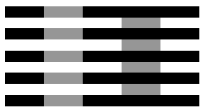
Here’s a classic contrast effect:

the same shade of grey looks darker when surrounded by white, than when surrounded by black.
For a long time psychology textbooks gave this as an example of a hardwired contrast effect – i.e. this is caused by the basic wiring of neurons in our eyes. (Some still do).
But take a look at this (White’s illusion):
here the same shade of grey looks lighter on the left than on the right, despite the surroundings being relatively lighter on the left than on the right. This is exactly the opposite of what’s predicted by a hardwired contrast effect in perception.
(An even cleaner example would be ceteris paribus, where making some part of the background lighter, all else held equal, makes the foreground appear lighter. The figure above does imply that there must exist at least one such case: imagine a third set of grey rectangles which are surrounded only by white. That third case must serve as a ceteris paribus case for one or other of the two cases above, probably both.)
The general point is this: There is not a stable relationship between the perceived-lightness of an object and the lightness of surrounding objects. There isn’t even an all-else-equal relationship. The relationship can run in either direction depending on the context.
But that’s not the last word. The set of contexts where it goes one way or the other way aren’t arbitrary (“contrast effects” and “assimilation effects”). Adelson (2001) shows that you can usually predict when you’ll observe one effect or the other: roughly, whether or not the surrounding lightness is a positive or negative ecological cue for illumination. I.e., in typical circumstances, is the surrounding lightness positively or negatively associated with illumination? (See an example at the bottom of this post.)
DIGRESSION 2
I would write out lists of comparison-effect examples over and over while working on my PhD. My train of thought would get detached and I’d end up asking myself questions like: What are you doing sitting in this office, a continent away from your friends and an ocean and a continent away from your family? Why do you spend your weekends in this sad building, where people stare at the carpet when they pass each other? What rock did you hit in adolescence that knocked you out of orbit, and sent you here? Are you trying to make your mother proud? Avenge your father? Do these professors you work with look like the kind of man you want to be? Did you stumble into one of those academic fields that people snigger about? Why, when you talk about your work, do the people you admire glaze over, and the people who bore you perk up? Do you think that giving your life to intellectual things makes you better than other people? Do you look down on people who don’t think so clearly? What are you doing on a Friday night at the NBER eating a tuna subway sandwich and reading reddit? If it takes you 5 years to get straight one point about relative thinking – one corner of one shelf in one cupboard – then how long is it going to take to tidy up the whole house? When an undergraduate corners you, asking earnest & tedious questions, doesn’t it remind you of yourself?

ALTERNATIVE HEURISTICS
OK. Well, here’s the body of the argument: I’m going to discuss a few perfectly reasonable reasons why we might infer the value of different attributes from the choice set, and each reason will imply one of the above laws in a subset of cases. However I also show that the same reason can imply the exact opposite of that law, for cases outside that subset.
(1) MRS shifting towards MRT.
A choice set which varies in different attributes has an implicit rate of tradeoff between the attributes – i.e. the marginal rate of transformation (MRT) – and it is easy to think of cases where our preferences would naturally adapt to the implicit tradeoff, i.e., where our relative value, AKA our marginal rate of substitution (MRS), would rotate towards the tradeoff that is implicit in the choice set (i.e. the MRT).
The MRS shifting towards the MRT could be rationalized in two separate ways. First, suppose you believe the social MRS to be informative about your own MRS, and you believe that the choice set reflects the market price, and finally that the price reflects the social MRS (as it would in a competitive equilibrium). Second, suppose you believe the person who constructed the choice set to be cooperative (in the sense of Grice) - i.e., they only include things in the choice set which they think you might want: this implies that the MRT in the choice set reflects their beliefs about your MRS, which is itself informative. If I’m staying in your spare room and and you ask me “would you prefer a poached egg or gruel for breakfast?” then I will figure that your gruel must be pretty good.
If there are just two attributes (i,j) and two alternatives (a,b) then the implicit tradeoff is \(MRT_{i,j}=\frac{\|a_{i}-b_{i}\|}{\|a_{j}-b_{j}\|}\). If the MRS rotates to meet this MRT then the sensitivity to attribute \(i\) will be decreasing in the range observed along that dimension, exactly as implied by the range-sensitivity theory (i.e., V, M&C, BR&S).
However the MRS-MRT effect implies range sensitivity only for a 2-attribute, 2-alternative case. Outside of that case the intuitions depart.
A marginal rate of transformation can only be directly identifed from a menu if the number of alternatives is equal to the number of attributes. I.e., to define a plane in \(n\) dimensions from a set of points, you’ll need exactly \(n\) points. If you have fewer then it becomes the statistical problem of fitting a line to a set of points. Here is a simple example where the MRT theory and other theories (e.g. range-sensitivity) give qualitatively different answers, and in which the MRS-MRT theory seems more faithful to the intuition. Suppose we have the following three options:
\[ \xymatrix@C=1em@R=1em{ & \binom{\mbox{100K salary}}{\mbox{199 days off}}\\ \\ & & \binom{\mbox{105K salary}}{\mbox{189 days off}} & \binom{\mbox{110K salary}}{\mbox{189 days off}}\\ \\ \ar[rrrr]\ar[uuuu] & & & & & \, \\ } \]
The intermediate option is dominated by the by the option on the right, and intuitively - to me - the existence of the intermediate option makes the rightmost option more desirable - because the choice set makes 10-days-off seem to be worth between \$5K and \$10K, meaning the higher salary seems to come at a low cost in terms of days-off. This intuition is not captured by range sensitivity, because the intermediate option does not change the range in either dimension. However the intermediate option does change the implicit MRS, in the sense of the best-fitting line (e.g. orthogonal regression), and the change will be in favor of the rightmost option – fitting my own intuition.
Even in the 3-attribute 3-alternative case, it is no longer true that \(MRT_{i,j}\) is equal to the ratio of ranges on dimension i and j, it’s now a more complicated function.
When one attribute is a good and the other is a bad (e.g. price and quality; salary and hours) it is sometimes reasonable to think that choosing neither alternative is an additional implicit element of the choice set, i.e. the point (0,0). In these cases the ratio of the ranges reduces to the ratio of the maximum values (\(\frac{\max_{c\in C}c_{i}}{\max_{c\in C}c_{j}}\)), which has similar comparative statics to the theory in (C) - which depends on the ratio of average values - than the theory in (V,M&C,BR&S) - which depends on the ratio of the ranges.
An interesting fact: the effects of this MRS-MRT theory will not be detectable when the choice set is binary: suppose your MRS shifts towards the MRT implicit in the choice set, then although your final MRS will be closer to the MRT, it will not cross the MRT, i.e. the shift in MRS will not alter which of the two elements you prefer. This implies that the MRS-MRT theory cannot rationalize the existence of cycles in binary choice, and so cannot explain evidence for ‘subadditivity’ of different dimensions, such as probability, money, or delay (see Read (2001) for citations). For example, if your have a prior belief that \(a\) is better than \(b\), and then you observe a choice set containing \(a\) and \(b\), then you may revise upward your valuation of \(b\) relative to \(a\), but this observation wouldn’t cause you to switch preference, i.e. to think that \(b\) is now better than \(a\). (This could be violated under some unusual priors, e.g. if you had bimodal beliefs about the value of \(b\)).
(2) MRS shifting towards demand.
There is a second strong intuition for choice sets influencing preferences: combinations offered often reflect combinations desired, so a relative increase in attribute 1 could be interpreted as a positive signal about the value of attribute 1. Suppose we manipulate the choice set, while keeping the relative price fixed, for example consider these two choice sets, trading off the price and quantity of some good:
\[ \xymatrix@C=.5em@R=.5em{\ar[rrrrr]\ar[ddddd] & & & & & \text{apples}\\ & \binom{\text{1 apple}}{\$1}\\ & & \binom{\text{2 apples}}{\$2}\\ & & & \binom{\text{3 apples}}{\$3}\\ \\ \\ \$ } \]
\[ \xymatrix@C=.5em@R=.5em{\ar[rrrrr]\ar[ddddd] & & & & & \text{apples}\\ & \,\,\,\,\,\, & \\ & & \binom{\text{2 apples}}{\$2}\\ & & & \binom{\text{3 apples}}{\$3}\\ & & & & \binom{\text{4 apples}}{\$4}\\ \\ \$ } \]
A natural intuition is that people will tend to switch from \(\binom{2}{\$2}\) to \(\binom{3}{\$3}\), when going from the first to the second choice set. None of the theories discussed above gives an unambiguous prediction about the change in MRS between these two choice sets - because both the range and magnitude change by the same amount on each dimension - yet the intuition remains quite clear (I think).
This idea could be easily formalized - suppose people know the supply curve but are uncertain about the demand curve - then when they observe an increase in quantity they attribute this to a higher demand, and so they infer an increase in value of the good. I think this is similar to the intuition given in Kamenica (2008) - when you observe a higher price/quantity combination, you infer that demand is higher, and so you infer that the value of each marginal good must be higher. I think that a similar foundation is used in Drolet, Simonson, Tversky (2000) “Indifference Curves that Travel with the Choice Set”.
We have discussed diagonal shifts along the budget set, meaning that both attributes are varying at once; if only one attribute varied, it’s not clear what a consumer would infer from this. Of course we could formalize a model where the consumer is uncertain about both supply and demand; or we could combine this model with the prior one, where the consumer is uncertain about the price.
(3) Magnitude effects.
Finally it’s easy to come up with a rational magnitude effect, such that when we observe a higher quantity \(q\) we infer that the marginal value of each unit is less. Suppose we know the price and we know the consumption-value of a good, when measured in units that are familiar to us, but we do not know the units that are used in the packaging. Then if we observe other people consuming a higher quantity, measured in unfamiliar units, we infer that each unit is worth less: when we observe a 10,000 Kronor bank note we infer each Kronor is not worth a lot; when we observe a 10,000 Watt bulb we infer each Watt is not worth much; when we observe 200mg of Oxytocin we infer the marginal effect of a milligram is not too much.
SUMMARY
When we dig into the intuitions behind comparison effects, we often find that they resemble inferences that we would make every day. The laws that have been proposed to explain comparison effects only work because they coincide with one or other of the inferences in certain subsets of cases – e.g. range-sensitivity coincides with MRS-MRT inference, magnitude-sensitivity coincides with unit-value inference. But these overlaps occur only in a subset of cases, and stepping outside that subset we find that the law fails, while the inference remains.
Does this mean that comparison effects are all just rational inferences? What we would like to know is whether comparison effects occur even when inference can be entirely ruled out – e.g. when we run an experiment that explicitly randomizes the choice sets. Some papers do this, but few do it well. I am persuaded that comparisons do affect us on a pre-conscious level, i.e. that our instincts latch onto comparisons without being careful about the significance of the comparison in the particular circumstance, but there’s not a lot of unambiguous evidence on this. I can at least say that most people find the types of example listed above pretty beguiling: they get strong intuitions about relative value, but struggle to explain where the intuitions come from, implying that the inference isn’t entirely conscious.
So then why would we make bad inferences that resemble good inferences? I think for the same reason that our perception makes bad inferences that resemble good inferences – because perceptual processes interpret cues according to their ordinary significance, without adjusting for all relevant information. Perception is carried out in a cabinet, whirring through the sense data, and printing out conclusions for the conscious mind to read. The cabinet is locked, we only have access to the output. That is the argument of my paper on ‘implicit knowledge’.
MISCELLANEOUS NOTES
It is useful to make a sharp distinction between “goods” and ’bads”. Examples of good-bad tradeoffs are quality vs price; salary vs hours worked. Examples of good-good tradeoffs are bedrooms vs bathrooms; MPG vs horsepower; salary vs holiday-days.
Parducci invented, as well as range-frequency theory, windsurfing.
Bordalo Gennaioli and Shleifer (2013) has a weird feature: the salience of an attribute depends on relative levels (\(q-\bar{q}\) and \(p-\bar{p}\)), but the utility of an attribute depends on absolute levels (\(q\) and \(p\)). I think this is just a mistake – the underlying intuition is matched much better if \(U(q,p) = \hat{\theta}_q(q-\bar{q}) + \hat{\theta}_p(p-\bar{q})\) instead of \(U(q,p) = \hat{\theta}_q q + \hat{\theta}_p p\). This alternation removes a lot of the weird comparative statics of the theory, such as the severe non-monotonicity of the decoy effects. Another note: for two-alternative two-attribute choices the theory (as stated in the paper) has a utility representation, i.e. many of the predictions of that paper are equivalent to a model with menu-independent preferences. For a sufficiently large value of \(M\):
\[ U(q,p)=\begin{cases} \delta q-p & ,\,q<\delta p\\ M+\ln q-\ln p & ,\delta p<q<\delta^{-1}p\\ M+q-\delta p & ,\,q>\delta^{-1}p \end{cases} \]

REFERENCES
KS: Koszegi and Szeidl (2011) (KS)
BRS: Bushong Schwarzstein & Rabin (2014)
MC: Mellers & Cooke (1994)
C: Cunningham (2013)
BGS: Bordalo Gennaioli Shleifer (2012)
Simonson (2008) “Will I like a Medium Pillow?”
“much of the evidence for preference construction reflects people’s difficulty in evaluating absolute attribute values and tradeoffs and their tendency to gravitate to available relative evaluations … These illustrations suggest that many forms of preference construction reflect a key underlying principle: decision makers tend to avoid absolute value judgments and gravitate to accessible relative evaluations … it is noteworthy that the evidence that has been accumulated to make the case for preference construction might be largely driven by a rather simple common principle. This rather simple, yet important absolute-to-relative principle lends itself to seemingly unrelated demonstrations, which have been treated as distinct phenomena and received unique labels.”
David Stove (1991) “What is Wrong With our Thoughts?”
Another Illusion
Adelson’s “steps” illusion:
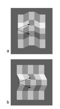
In the first picture the two squares with arrows on them look similar, but in the second picture they seem to have different shades. They are (as you guessed) all the same shade, and in fact the shades are all identical between the first and second image, just arranged a little differently.
In particular, the tilt gives an the impression of an angle, and so influences our judgment of where the illumination is coming from. In the first image both squares seem to be on the same plane; in the second image the upper square seems to be on a plane with light squares, and the lower square seems to be on a plane with dark squares. If we use, as proxies of illumination for a square, the shade of squares coplanar with it, then we get the predicted effect.
More Examples
- If you have to judge the value of 10 of something – say you’re bidding on 10 bottles of wine in an auction – they’ll seem more valuable if, at the same time, you’re also considering a single bottle of wine; and vice versa if you’re also considering 100 bottles of wine.
- If you’re choosing between a low-price and medium-price version of a good, seeing that there’s also a high-price version makes the medium-price version seem relatively more attractive.
- (See my ‘comparisons and choice’ paper for more examples).
Citation
@online{cunningham2016,
  author = {Cunningham, Tom},
  title = {Relative {Thinking}},
  date = {2016-04-30},
  url = {https://tecunningham.github.io/posts/2016-04-30-relative-thinking.html},
  langid = {en}
}