LLM Time-Saving and Demand Theory

Suppose an LLM speeds you up by factor \(\beta\) on tasks that are a share \(s\) of your time.

What is your overall increase in output for a given time? Should we expect it to be \(s\times(\beta-1)\), or larger or smaller?

How does the answer change if you measure the time-share \(s\) before vs after you start using LLMs?

If we can observe the time-shares both before and after LLMs, does that help with estimating the overall efficiency gain?

Economic theory has crisp answers to these questions.

These questions are all equivalent to classic economic questions of how people change expenditure in response to changes in prices. Below I give a cheat sheet, a lookup table, derivations, and some brief survey of different relevant literatures (there are surprisingly many related literatures).

My guess is that LLMs are mostly substitutes.

LLMs let me complete 16 hours of work in an 8 hour day, but the LLM is mostly accelerating me on things that I wouldn’t otherwise spend my time on (e.g. fact checking, literature reviews, visualizations), meaning they are substitutes, and so my effective productivity lift is much lower than a doubling of time.

Cheat Sheet

Assume people spend their time rationally.

We will assume people allocate time between sped-up and non-sped-up tasks rationally, trying to maximize their overall output.

The output gain will be between \(\frac{1}{(1-s)+s/\beta}\) and \(\beta\).

We can put upper and lower bounds on the effect on aggregate output (for a fixed time input):

1. If the tasks are perfect substitutes: \(\beta\).
2. If the tasks are perfect complements: \(\frac{1}{(1-s)+s/\beta}\)

The percent gain is simple in two cases.

We can apply the small-change approximation \(y'/y \approx 1 + s(\beta-1)\) if either of two cases holds:

1. Most tasks are affected by the speedup (\(s\simeq 1\))
2. The productivity increase is small (\(\beta\simeq 1\)) (AKA Hulten’s theorem)

In these two cases we can estimate the aggregate productivity improvement without knowing the degree of substitutability between tasks.

If the time-savings are somewhat small then you can use elasticity of substitution.

If you know the elasticity of substitution between sped-up tasks and other tasks, \(\varepsilon\), then we can write an expression for the aggregate increase: \[\frac{y'}{y} = \left((1-s) + s\,\beta^{\varepsilon-1}\right)^{1/(\varepsilon-1)}\]

If the time-savings are large, use the area under the demand curve.

If the time-savings are large then it’s more dangerous to assume a constant elasticity. Instead we ideally want to trace out the entire demand curve (i.e. how time-allocated to a task changes as the efficiency increases), and the speed-up will be proportional to the area under the demand curve.

Using pre-LLM shares will under-estimate value for substitutes (and over-estimate for complements).

If using the simple \(s\times(\beta-1)\) estimate, then using pre-LLM shares will under-estimate productivity improvements when tasks are substitutes, while using post-LLM time-shares will over-estimate; the direction flips when tasks are complements.

Observing pre-LLM and post-LLM shares helps.

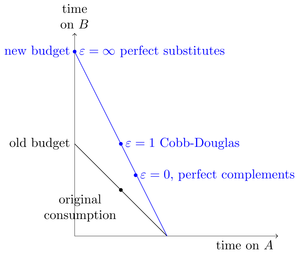
If you observe the time-share both pre-LLM and post-LLM then you can back out the elasticity of substitution, and thus the aggregate efficiency improvement. Graphically, if we observe the change in budget constraint, and change in consumption point, we can infer substitutability, and therefore aggregate productivity improvement.

Applications

Estimating productivity improvements from query-level time-savings.

Anthropic (2025) samples a range of tasks from Claude chatbot logs and estimates the time required for each task both with and without AI assistance.

My understanding of their calculation:

1. Claude is used for around 25% of tasks, \(s=0.25\) (pre-LLM distribution of tasks).
2. When Claude is used, time-required falls by 80%, \(\beta=5\).
3. Therefore the total time-saving is around 20% (using the fixed-share calculation \(s(1-1/\beta)\) with these numbers; this is the small-change/Hulten-style approximation).

However as we discussed above, Hulten’s theorem only applies for small efficiency changes, but these are large changes (80%), so this conclusion requires assuming Cobb-Douglas substitution, i.e. that time-shares are constant.

==my guess: people are doing tasks they wouldn’t otherwise do.==

Estimating time-savings in an RCT.

Becker et al. (2025) report an RCT, where software engineers first choose tasks, then get assigned to either with-AI or without-AI conditions. In this case the subjects mostly were not using AI, but in follow-up studies they will be using AI. This makes it hard to think about interpreting uplift studies over time, insofar as AI causes them to change the task distribution. It would be nice to have a good clear language here.

Lookup Tables

Output increase using ex-ante time shares

	1.1X speedup on 50%	2X speedup on 10%	5X speedup on 10%
\(\varepsilon=0\) (perfect complements/Amdahl)	4.8%	5.3%	8.7%
\(\varepsilon=1/2\) (complements)	4.8%	6.1%	12.0%
\(\varepsilon=1\) (Cobb-Douglas/Hulten)	4.9%	7.2%	17.5%
\(\varepsilon=2\) (substitutes)	5.0%	10.0%	40.0%
\(\varepsilon\rightarrow\infty\) (perfect substitutes)	10.0%	100.0%	400.0%

Output increase using ex-post time shares:

	1.1X speedup on 50%	2X speedup on 10%	5X speedup on 10%
\(\varepsilon=0\) (perfect complements/Amdahl)	5.0%	10.0%	40.0%
\(\varepsilon=1/2\) (complements)	4.9%	8.5%	26.2%
\(\varepsilon=1\) (Cobb-Douglas/Hulten)	4.9%	7.2%	17.5%
\(\varepsilon=2\) (substitutes)	4.8%	5.3%	8.7%
\(\varepsilon\rightarrow\infty\) (perfect substitutes)	N/A	N/A	N/A

How these are calculated:

• “X% saving” means task-2 productivity increases so that time-per-unit falls by factor \((1-X)\), i.e., \(\beta = 1/(1-X)\). So 10% saving → \(\beta = 1.11\); 50% saving → \(\beta = 2\); 80% saving → \(\beta = 5\).
• “Y% of work” means the time share on task 2 is \(s = Y\).
• Output gain from the CES formula: \[\frac{y'}{y} = \left((1-s_0) + s_0\,\beta^{\varepsilon-1}\right)^{1/(\varepsilon-1)}\] where \(s_0\) is the ex-ante share. The reported numbers are \((y'/y-1)\times 100\%\).
• Table 1: The column header specifies the ex-ante share \(s_0\) directly. Compute the output gain and report the percent increase.
• Table 2: The column header specifies the ex-post share \(s_1\). First back out the implied ex-ante share using: \[\frac{s_0}{1-s_0} = \frac{s_1}{1-s_1} \cdot \beta^{1-\varepsilon}\] Then compute the true output gain using \(s_0\).
• Perfect substitutes (Table 2): After any productivity improvement, you reallocate entirely to the better task, so the ex-post share is always 100%. Specifying it as 10% or 50% is inconsistent with optimization—hence N/A.

Other Points

An analogy: we’re turning lead into gold.

Suppose I invent a technology to turn lead into gold, so that the price of gold falls by 99%. I’d like to quantify my welfare increase in terms of equivalent income. I could apply a simple share-weighted price-change rule in two ways:

1. If I use ex ante expenditure the effect looks small: my expenditure share on gold is ~0%, so even a 100% price decrease has a negligible effect on my effective income.

2. If I use ex post expenditure the effect looks large: if gold is sufficiently cheap then I’ll start buying many things which are made of gold. Suppose I now spend 1% of my income on gold, then it looks like the price reduction has doubled my effective income, because at the original price of gold I would’ve had to have twice as much income to afford my new basket.

This discrepancy between ex ante and ex post values arises because of the high substituability between gold and other materials (steel, bronze). However I’m not confident that we would see that elasticity at current prices, it would only occur when gold’s price gets sufficiently low, meaning that estimating a CES function wouldn’t be sufficient to give a good estimate of the value. To get a realistic estimate we need to map elasticities at different prices, i.e. draw the entire demand function.

Sensitivity to CES.

I give bounds on aggregate time-savings with a CES model below, but I’m not sure whether you’d get wider bounds if you relax the CES assumption, e.g. account for second-order effects.

Non-homotheticities.

In demand theory there can be significant effects from non-homotheticities.

Tasks are fake.

(…)

Model

We set up a two-task CES production problem and derive the optimal time split, the implied output, and the response to productivity changes, with limits for common special cases.

Practical implications (at a glance)

Let \(s\equiv t_2^*\) denote the optimal time share on task 2 (and \(1-s=t_1^*\)). Express all effects as log-changes \(\Delta\ln y^*=\ln\!\big(y^{*'}/y^*\big)\) when task-2 productivity moves from \(A_2\) to \(A_2'=\beta A_2\). The last column plugs in \(s=0.1\) and \(\beta=2\).

Case	Output effect (\(\Delta\ln y^*\))	Intuition	Example \(\Delta\ln y^*\) (\(s=0.1,\ \beta=2\))
General finite change	\(\dfrac{1}{\varepsilon-1}\ln\!\big((1-s)+s\,\beta^{\varepsilon-1}\big)\)	CES-weighted average of the shock	\(\dfrac{1}{\varepsilon-1}\ln\!\big(0.9+0.1\times2^{\varepsilon-1}\big)\) (depends on \(\varepsilon\))
Perfect substitutes (\(\varepsilon\rightarrow\infty\))	\(\ln \beta\)	All time moves to the better task	\(\approx 0.69\)
Cobb–Douglas (\(\varepsilon=1\))	\(s\,\ln \beta\)	Log-linear weighting by the task share	\(\approx 0.069\)
Perfect complements (\(\varepsilon\rightarrow0\))	\(-\ln\!\big((1-s)+s/\beta\big)\)	Bottlenecked by the slow task	\(\approx 0.051\)
Infinitesimal change (Hulten)	\(s\,d\ln A_2\)	Percent gain equals time share on improved task	\(0.1\times\ln 2\approx 0.069\)

Setup and parameters

• Time endowment is \(1\); choose \(t_1\in[0,1]\) and \(t_2=1-t_1\).
• Productivities: \(A_1>0\) for task \(1\), \(A_2>0\) for task \(2\).
• Taste weight: \(\alpha\in(0,1)\) on task \(1\).
• Substitution parameter: \(\varepsilon>0\); take \(\varepsilon\neq1\) for the algebra and then send \(\varepsilon\rightarrow1\) for the Cobb–Douglas limit.
• Output aggregator (CES): \[y(t_1,t_2)=\left(\alpha(A_1 t_1)^{\frac{\varepsilon-1}{\varepsilon}}+(1-\alpha)(A_2 t_2)^{\frac{\varepsilon-1}{\varepsilon}}\right)^{\frac{\varepsilon}{\varepsilon-1}}.\]

Assumptions

1. Feasible set: \(t_1\in[0,1]\), \(t_2=1-t_1\).
2. Parameters satisfy \(A_i>0\) and \(\alpha\in(0,1)\).
3. Decision problem: choose \(t_1\) to maximise \(y(t_1,1-t_1)\).

Proposition 1 (optimal time split). The interior optimum is \[t_1^*=\frac{1}{1+\left(\frac{1-\alpha}{\alpha}\right)^{\varepsilon}\left(\frac{A_2}{A_1}\right)^{\varepsilon-1}},\qquad t_2^*=1-t_1^*.\]

Proof (explicit)

1. Write the Lagrangian \(\mathcal{L}=y(t_1,t_2)+\lambda(1-t_1-t_2)\) with \(y\) as above.
2. First-order conditions (interior): \(\partial\mathcal{L}/\partial t_1=0\) and \(\partial\mathcal{L}/\partial t_2=0\) give \[\lambda=\alpha\,A_1^{\frac{\varepsilon-1}{\varepsilon}}\,t_1^{-\frac{1}{\varepsilon}}\,y^{\frac{1}{\varepsilon}}=(1-\alpha)\,A_2^{\frac{\varepsilon-1}{\varepsilon}}\,t_2^{-\frac{1}{\varepsilon}}\,y^{\frac{1}{\varepsilon}}.\]
3. Cancel \(y^{\frac{1}{\varepsilon}}\) and rearrange to obtain \(\frac{t_2}{t_1}=\left(\frac{1-\alpha}{\alpha}\right)^{\varepsilon}\left(\frac{A_2}{A_1}\right)^{\varepsilon-1}\).
4. Impose \(t_1+t_2=1\) and solve for \(t_1^*\); set \(t_2^*=1-t_1^*\).
5. The interior solution is valid for \(\varepsilon>0\) with finite \(A_i\); only the perfect-substitutes limit \(\varepsilon\rightarrow\infty\) or \(A_i\rightarrow0\) forces a corner.

Proposition 2 (indirect output). At \(t_1^*,t_2^*\) the output is \[y^*=\Big(\alpha^{\varepsilon}A_1^{\varepsilon-1}+(1-\alpha)^{\varepsilon}A_2^{\varepsilon-1}\Big)^{\frac{1}{\varepsilon-1}}.\]

Proof (explicit)

1. Substitute \(t_1^*,t_2^*\) from Proposition 1 into \(y(t_1,t_2)\).
2. Factor out \(\alpha^{\varepsilon}A_1^{\varepsilon-1}+(1-\alpha)^{\varepsilon}A_2^{\varepsilon-1}\) inside the braces; the exponent \(\frac{\varepsilon}{\varepsilon-1}\) collapses to the stated form.

Proposition 3 (infinitesimal productivity change). Holding \(A_1\) fixed, a small change in \(A_2\) satisfies \[\frac{dy^*}{y^*}=t_2^*\,\frac{dA_2}{A_2}.\]

Proof (explicit)

1. Take \(\log y^*=\frac{1}{\varepsilon-1}\log\big(\alpha^{\varepsilon}A_1^{\varepsilon-1}+(1-\alpha)^{\varepsilon}A_2^{\varepsilon-1}\big)\).
2. Differentiate with respect to \(\log A_2\): \[\frac{dy^*}{y^*}=\frac{(1-\alpha)^{\varepsilon}A_2^{\varepsilon-1}}{\alpha^{\varepsilon}A_1^{\varepsilon-1}+(1-\alpha)^{\varepsilon}A_2^{\varepsilon-1}}\cdot\frac{dA_2}{A_2}.\]
3. The fraction equals \(t_2^*\) from Proposition 1, so the result follows.

Proposition 4 (finite productivity change on task 2). If \(A_2'=\beta A_2\) with \(\beta>0\), then \[\frac{y^{*'}}{y^*}=\left(t_1^*+(1-t_1^*)\beta^{\varepsilon-1}\right)^{\frac{1}{\varepsilon-1}}.\]

Proof (explicit)

1. Replace \(A_2\) by \(\beta A_2\) in \(y^*\) from Proposition 2: \[y^{*'}=\Big(\alpha^{\varepsilon}A_1^{\varepsilon-1}+(1-\alpha)^{\varepsilon}(\beta A_2)^{\varepsilon-1}\Big)^{\frac{1}{\varepsilon-1}}.\]
2. Factor out the old level \(y^*\) to form a ratio; the remaining weights inside the braces are \(t_1^*\) and \(t_2^*=1-t_1^*\), giving the stated expression.

Proposition 5 (canonical limits). Take limits of Proposition 4:

• Cobb–Douglas (\(\varepsilon\rightarrow1\)): \(\frac{y^{*'}}{y^*}\rightarrow \beta^{1-\alpha}\) and \(t_i^*\) is unchanged.
• Perfect complements (\(\varepsilon\rightarrow0\)): \(\frac{y^{*'}}{y^*}\rightarrow \frac{1}{t_1^*+t_2^*/\beta}\).
• Perfect substitutes (\(\varepsilon\rightarrow\infty\)): \(\frac{y^{*'}}{y^*}\rightarrow \beta\) with \(t_2^*\rightarrow1\) if \(\beta A_2>A_1\).

Proof sketch For \(\varepsilon\rightarrow1\) apply L’Hôpital to the CES form. For \(\varepsilon\rightarrow0\) the CES aggregator converges to \(\min\{A_1 t_1,A_2 t_2\}\). For \(\varepsilon\rightarrow\infty\) it converges to \(\max\{A_1 t_1,A_2 t_2\}\). Substitute these limits into Proposition 4 and simplify.

Related Theory

I don’t consider myself an expert on these literatures, take this survey at your own risk.

The index numbers problem.

There’s a very old literature on calculating an aggregate price index in a way that accounts for substitutability between different goods. The same theory can be applied to change in goods-prices or task-productivities, see Caves, Christensen, and Diewert (1982).

• The Laspeyres index uses base-period weights, and will understate gains when a shock makes you reallocate toward the lower-price good.

• The Paasche index uses end-period weights, and will overstate gains when a shock makes you reallocate toward the lower-price good.

• A Divisia index is a path integral of share-weighted growth rates. Discrete indices (e.g., Fisher/Törnqvist) are designed to approximate that integral.

Consumer surplus / welfare for large “price” (time-cost) changes

The classic consumer surplus measure from a price change is the area under the demand curve, however this measures the Marshallian consumer surplus, which will approximate the welfare-relevant Hicksian surplus only when there are negligible income effects. Willig (1976) gives approximation bounds.

This literature distinguishes between Equivalent Variation (EV), the change in income that would have the same welfare effect as the price change, and Compensating Variation (CV), the change in income which could accompany the price change and restore your utility.

Hausman (1981) shows how to compute exact welfare measures (EV/CV, deadweight loss) from an estimated demand curve by imposing integrability (i.e., that the demand actually comes from some underlying utility/expenditure function). Deaton and Muellbauer (1980) provides a standard integrable demand system (AIDS) that flexibly captures income and substitution patterns.

Economics of time allocation (time is a scarce input with shadow prices)

DeSerpa (1971) is a classic reference on time allocation, and time-saving innovations as relaxing the budget constraint.

Task substitution and computerization as task-specific technology shocks

Autor, Levy, and Murnane (2003) gives the modern “tasks” approach: computerization substitutes for routine tasks and complements non-routine tasks, shifting task content within occupations and generating distributional consequences (e.g., polarization). You cannot summarize tech change as “labor-augmenting” in the aggregate.

Acemoglu and Autor (2011) synthesizes and formalizes this task-based view. A central message is that the impact of a task-specific productivity shock depends on: (i) which tasks are affected, (ii) how substitutable tasks are, and (iii) how the economy re-optimizes task assignment across workers/technologies.

Hulten’s theorem and when first-order share-weighting breaks

Hulten (1978) shows (in a competitive, CRS setting with intermediates) that a small productivity shock’s effect on aggregate productivity can be summarized by share-weighted sectoral TFP growth (Domar/revenue-share weights). The key takeaway is the legitimacy of first-order share weighting—but only locally.

Baqaee and Farhi (2019) shows that in production networks, micro shocks can have macro consequences and nonlinearities/higher-order terms matter.

Baqaee and Burstein (2021) and Comin, Lashkari, and Mestieri (2021) take into account income effects.

Amdahl’s law as the perfect-complements benchmark

Amdahl’s law in computer science says the speedup from improving one component is bounded by the unimproved fraction. This corresponds to the perfect-complements case.

Illustrations

Indifference Curve

Budget constraint and optimal allocations under different elasticities

Demand Curve

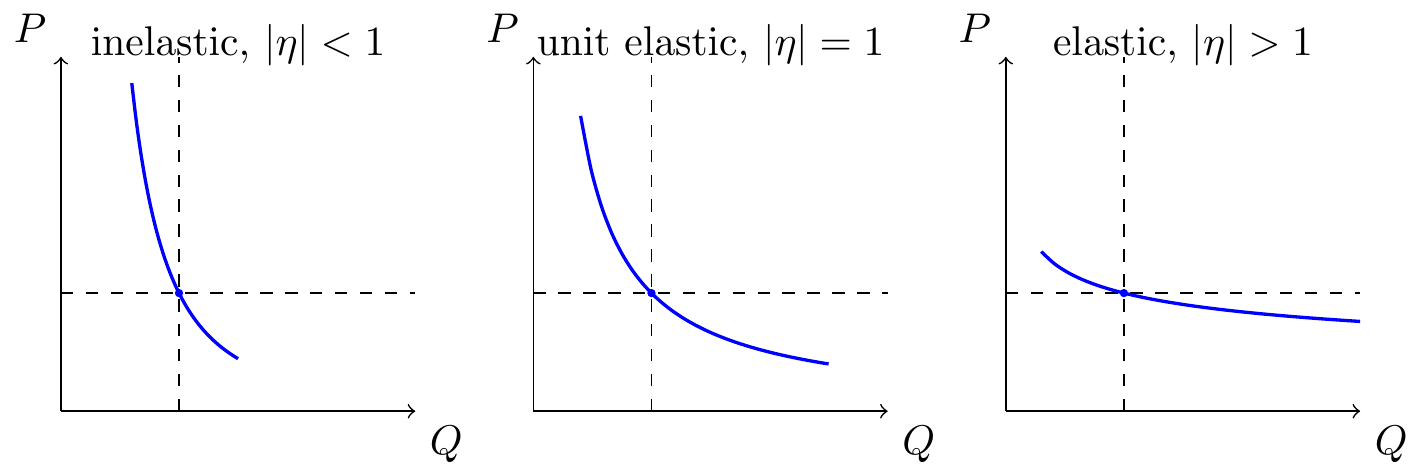
Demand curves with different price elasticities

2026-01-17 | AI & substitution

Puzzle:

1. Task speedups bigger than aggregate speedups. LLMs seem to be having large speedups for tasks that make up a large share of peoples’ time, yet this doesn’t seem to reflect actual productivity.
2. Resolution: LLMs are mostly making new tasks affordable, rather than lowering the cost of existing tasks. It’s like making a Cadillac the same cost as a Toyota, instead of lowering the cost of all cars uniformly.
3. How to test this. We want to know the effects of LLMs on both (A) task speed; (B) task selection.
   • Ask people which tasks they would select with & without AI.
   • Add a time cost to tasks. See how task selection will change if you add artificial time costs, e.g. you have to do CAPTCHA for 1 minute.
   • Observe effect of latency.
4. Note: elasticity of substitution not useful.

Mathematically:

1. Unit demand. There are \(n\) different tasks, each has payoff \(u_i\) and time-cost \(p_i\). \[\begin{aligned} U &= \sum_{i=1}^n u_i \times \mathbb{1}\{t_i\geq p_i\} \\ \sum_i^n t_i &= 1 \end{aligned} \] If the time-cost of existing tasks falls by \(1/\beta\) then utility increases by \(\beta\). But if the time-cost of new tasks (that you’re not already doing) falls then the utility increase is much less than \(1/\beta\). This is especially true if there’s a minimum time-cost to doing a task, e.g. every task takes at least 15 minutes.

2. Two quality levels. There \(n\) different activities, and two qualities, \(L\) and \(H\). The two quality-levels are perfect substitutes: \[\begin{aligned} U &= \sum_{i=1}^n\left( (x_{i,L}+x_{i,H})^\eta \right)^{1/\eta} \\ \end{aligned} \]

How to test:

1. SWE tasks.
   • Write out all tasks, check which ones you would do with Human vs Augmented.
   • Add a time cost to each task – you have to fill out CAPTCHA for 5 minutes.
2. Chatbot.
   • Add a latency cost.

concrete examples

1. Tom doing literature reviews. Suppose I spend 5 minutes each day using ChatGPT to do literature reviews, & the reviews would’ve taken me 8 hours to do without ChatGPT’s help, meaning this is a roughly 100X speedup. On the surface this seems to be doubling my aggregate productivity, i.e. I’m now doing 16 hours work in an 8 hour day.

   To get the true time-saving we need to know how substitutable these tasks (literature reviews) are for other tasks. Suppose for argument that ChatGPT hasn’t changed the share of my time I’m spending on literature reviews, it’s just made me far more productive. This implies an elasticity of substitution of 1. It also implies that

References

Acemoglu, Daron, and David Autor. 2011. “Skills, Tasks and Technologies: Implications for Employment and Earnings.” In, edited by David Card and Orley Ashenfelter, 4:1043–1171. Handbook of Labor Economics. Elsevier. https://doi.org/https://doi.org/10.1016/S0169-7218(11)02410-5.

Anthropic. 2025. “Estimating AI Productivity Gains from Claude Conversations.” 2025. https://www.anthropic.com/research/estimating-productivity-gains.

Autor, David, Frank Levy, and Richard J Murnane. 2003. “The Skill Content of Recent Technological Change: An Empirical Exploration.” The Quarterly Journal of Economics 118 (4): 1279–1333. https://doi.org/10.3386/w8337.

Baqaee, David Rezza, and Ariel Burstein. 2021. “Welfare and Output with Income Effects and Demand Instability.” Working Paper. https://www.semanticscholar.org/search?q=Welfare%20and%20Output%20with%20Income%20Effects%20and%20Demand%20Instability.

Baqaee, David Rezza, and Emmanuel Farhi. 2019. “The Macroeconomic Impact of Microeconomic Shocks: Beyond Hulten’s Theorem.” Econometrica 87 (4): 1155–1206. https://doi.org/10.3982/ecta15202.

Becker, Joel, Nate Rush, Elizabeth Barnes, and David Rein. 2025. “Measuring the Impact of Early-2025 AI on Experienced Open-Source Developer Productivity.” https://arxiv.org/pdf/2507.09089.pdf.

Caves, Douglas W., Laurits R. Christensen, and W. Erwin Diewert. 1982. “The Economic Theory of Index Numbers and the Measurement of Input, Output, and Productivity.” Econometrica 50 (6): 1393–1414. https://www.jstor.org/stable/1913382.

Comin, Diego, Danial Lashkari, and Martı́n Mestieri. 2021. “Structural Change with Long-Run Income and Price Effects.” Working Paper. https://doi.org/10.3982/ecta16317.

Deaton, Angus, and John Muellbauer. 1980. “An Almost Ideal Demand System.” American Economic Review 70 (3): 312–26. https://www.semanticscholar.org/search?q=An%20Almost%20Ideal%20Demand%20System.

DeSerpa, Allan C. 1971. “A Theory of the Economics of Time.” The Economic Journal 81 (324): 828–46. https://doi.org/10.2307/2230320.

Hausman, Jerry A. 1981. “Exact Consumer’s Surplus and Deadweight Loss.” American Economic Review 71 (4): 662–76. https://www.semanticscholar.org/search?q=Exact%20Consumer%27s%20Surplus%20and%20Deadweight%20Loss.

Hulten, Charles R. 1978. “Growth Accounting with Intermediate Inputs.” The Review of Economic Studies 45 (3): 511–18. https://doi.org/10.2307/2297252.

Willig, Robert D. 1976. “Consumer’s Surplus Without Apology.” American Economic Review 66 (4): 589–97. https://www.semanticscholar.org/paper/745fa39279d59c6f6b14dce4a38bcf098774c2ad.

Footnotes

1. with many thanks to Elsie Jang

2. with many thanks to Elsie Jang

3. with many thanks to Elsie Jang